How do you store and traverse a graph?.

Graphs

A graph is a non-linear data structure of nodes and edges. More formally:

A graph consists of a finite set of vertices (or nodes) and a set of edges which connect a pair of nodes.

Graphs model networks — paths in a city, telephone networks, circuits — and social networks like LinkedIn and Facebook, where each person is a vertex carrying info like id, name, and gender.

Example

If the following graph is a network of friends, then:

• Node 2 and 1 are friends.
• Node 2 and 4 aren’t (they are mutual friends of 1 and 3).

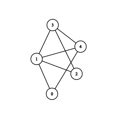
In this undirected graph, vertices V = {0,1,2,3,4} and edges E = {(1, 0), (0, 4), (1, 4), (1, 3), (3, 4), (1, 2), (3, 2)}.

Representations

A graph has two components:

1. A finite set of vertices (nodes).
2. A finite set of ordered pairs (u, v) called edges. The pair is ordered because (u, v) is not (v, u) in a directed graph. Edges may carry weight/value/cost.

The two most common representations are adjacency matrix and adjacency list (others: incidence matrix/list). The choice is situation-specific — it depends on the operations and ease of use.

Adjacency matrix

• A 2D array of size V × V. adj[i][j] = 1 means an edge from i to j.
• Always symmetric for undirected graphs.
• Weighted graphs: adj[i][j] = w means edge i → j with weight w.

The adjacency matrix for the example graph:

Pros:

• Easier to implement and follow.
• Removing an edge takes $O(1)$.
• Edge-existence queries (u → v?) take $O(1)$.

Cons:

• Space $O(N^2)$, even for sparse graphs.
• Adding a vertex costs $O(N^2)$.

Adjacency list

• An array of lists, one per vertex; array[i] holds vertices adjacent to i. Weights ride along as pairs.

Pros:

• Saves space: $O(|V|+|E|)$.
• Adding a vertex is easier.

Cons:

• Edge-existence queries cost $O(N)$.

Important terms

• Two nodes are connected if a path exists between them. Example: 1->2->3->4, so 1 and 4 are connected. Connectivity is defined via paths.
• Cycle: we return to the same node without repeating. Example: 1->2->3->4->1.
• Distance: number of edges between 2 connected nodes on the path. Example: 1->2->3->4 has distance 3.

Types of graphs

• Undirected graph: edges are non-directional. Example: Brother 1 ↔ Brother 2 [1 -- 2].
• Directed graph: edges are directional. Example: Father → Son, 1 --> 2.
• Weighted graph: edges have weights. Example: flight routes with costs.
• Unweighted graph: plain edges.
• Cyclic graph: has at least one cycle. Acyclic graph: otherwise.
• Connected graph: a path exists between any two nodes. Disconnected graph: otherwise — it has multiple connected components.

Trees and forests

• Both are acyclic — no cycles allowed.
• Tree: the graph is connected.
• Forest: the graph is disconnected — a collection of trees.

Connected components

1. In a connected component, all nodes are connected to each other.
2. A component must be maximal — not part of something bigger.

Connectivity check

Tell whether a given graph is connected or not.

Start at some vertex and follow edges — you must reach all other vertices.

How to store a graph in a program?

We need to know which vertex connects to which others.

1. Adjacency matrix adj[][] (discussed above).
2. Adjacency list (discussed above) — uses less memory.

DFS (depth first search)

Mark uncolored nodes with some color and count them; if the count equals the number of nodes, the graph is connected. Just like throwing popcorn in a maze to find the exit — a grid is just a graph whose nodes are positions we can move to.

DFS can also find the actual path between two nodes while checking it exists.

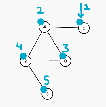
Algorithm:

count = 0

dfs(node):
    color[node] = blue; count++
     # Takes list for a vertex from adj list
    for X in adj[node]:
        if color[X] = blue:
            continue
        # Recursively go through all connected nodes
        dfs(X)

Code (C++):

const int N = 1'00'000;  // maximum number of nodes
vector<int> adj[N];      //adjacency list
bool visited[N];
int cnt;

void dfs(int node) {
    // mark it blue
    visited[node] = true;
    cnt++;
    for (int x : adj[node]) {
        if (visited[x]) continue;
        dfs(x);
    }
}

int main() {
    int n;  // nodes
    cin >> n;
    int m;  // edges
    cin >> m;
    for (int i = 0; i < m; ++i) {
        int x, y;
        cin >> x >> y;  // represents edge between x and y
        adj[x].push_back(y);
        adj[y].push_back(x);
        // As undirected so both edges
    }
    dfs(1);  // dfs from any node
    if (n == cnt) {
        // connected graph
    } else {
        // not connected
    }
    return 0;
}

What is the time complexity of DFS?

O(m + n) for m edges and n nodes.

Why?

Each node is visited once (never revisit a marked node) — so why not just O(n)? Because each edge is visited twice: at node A via A->B, and at node B via B->A. So n + 2*m reduces to O(n+m).

Connected components

Count the connected components in a given graph.

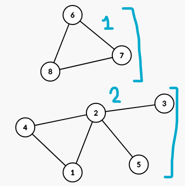
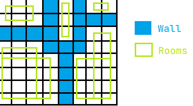
Example: counting rooms in a given area.

Algorithm:

components = 0

loop node from 1 to n:
    if node is blue:
        continue
    dfs(node)          #This function will look same
    components += 1

Find the number of rooms in this building map (CSES 1192):

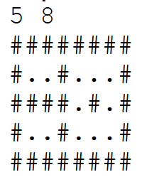
Code (C++):

int dx[] = {0, 0, 1, -1};
int dy[] = {1, -1, 0, 0};

int n, m;
bool visited[1010][1010];
char grid[1010][1010];

bool isValid(int x, int y) {
    if (y < 0) return false;
    if (x < 0) return false;
    if (y >= m) return false;
    if (x >= n) return false;
    if (grid[x][y] == '#') return false;
    return true;
}

void dfs(int x, int y) {
    visited[x][y] = true;
    for (int i = 0; i < 4; i++) {
        int X = x + dx[i];
        int Y = y + dy[i];
        if (isValid(X, Y)) {
            if (!visited[X][Y]) {
                dfs(X, Y);
            }
        }
    }
}

void CountingRooms() {
    cin >> n >> m;
    for (int i = 0; i < n; i++) {
        for (int j = 0; j < m; j++) {
            cin >> grid[i][j];
            visited[i][j] = 0;
        }
    }
    int components = 0;
    for (int i = 0; i < n; i++) {
        for (int j = 0; j < m; j++) {
            if (grid[i][j] == '.' && !visited[i][j]) {
                dfs(i, j);
                components++;
            }
        }
    }
    cout << components;
}

Methods of graph traversal

Two algorithms:

1. DFS (depth first search) — discussed above.
2. BFS (breadth first search).

Traversal order, side by side:

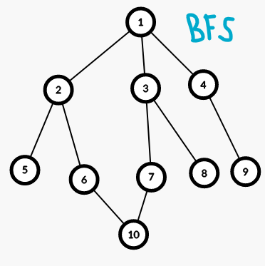
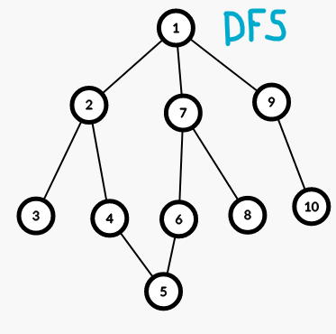
Uses of BFS

1. Shortest distance between 2 nodes.
2. Fix a node, find shortest distances to all others.
3. Find predecessors/parents, then backtrack the shortest path between two nodes.

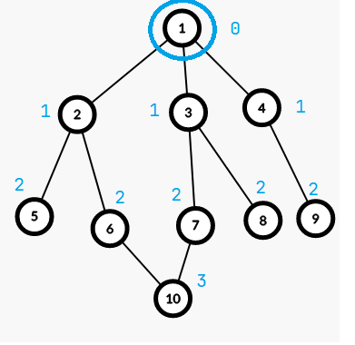
Example: shortest path between two houses in a city.

Algorithm

#A queue is used to store the order in which we visit vertices
queue
push initial vertex
distance[initial] = 0
while queue not empty:
    take front of queue
    add all unvisited children to queue
    mark distance

Code (C++)

const int N = 1'00'000;  // maximum number of nodes
vector<int> adj[N];      //adjacency list
int dis[N];
bool pushed_in_queue[N];  // visited

int main() {
    int n;  // nodes
    cin >> n;
    int m;  // edges
    cin >> m;

    for (int i = 0; i < m; ++i) {
        int x, y;
        cin >> x >> y;  // represents edge between x and y
        // Undirected
        adj[x].push_back(y);
        adj[y].push_back(x);
    }

    // lets say we have to run bfs from 1
    queue<int> q;
    q.push(1);  // fixed vertex
    dis[1] = 0;
    pushed_in_queue[1] = true;

    while (!q.empty()) {
        int node = q.front();  // currently visiting this node
        q.pop();               // dont want to visit this again

        // Go through all children
        for (int x : adj[node]) {
            if (pushed_in_queue[x] == true) continue;
            q.push(x);  //visit x later
            dis[x] = dis[node] + 1;
            pushed_in_queue[node] = true;  // to make sure we dont visit twice
        }
    }

    cout << dis[10];  // must be 3

    return 0;
}

What is the time complexity of BFS?

O(n + m) — every vertex is pushed and popped once, and every edge is visited twice, same as DFS.

Multisource BFS

In an unweighted graph, this is the fastest way to visit all nodes starting from the “special” nodes. Use it to find unvisited nodes, shortest-path lengths, or the paths themselves.

Oranges problem: green means rotten, orange means ripe. Every ripe orange adjacent to a rotten one rots in a minute.

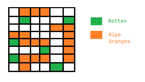
Q1. Will all oranges rot?

Yes here — but how to check in code? Treat oranges as graph vertices: every connected component must contain at least one rotten orange, so basic DFS answers it.

Q2. Assuming all rot, what is the minimum time?

Method 1: O(NM*NM). BFS from each ripe orange to the nearest rotten one costs O(NM); with up to NM vertices, total O(NM*NM).

Method 2: O(NM) — multisource BFS.

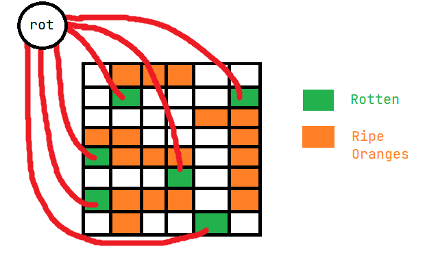
Imagine a node “rot” connected to all rotten oranges. BFS from “rot” gives every node’s minimum distance, and dist[i] - 1 is the distance from the nearest rotten orange. The maximum distance is the time taken.

So BFS runs once: O(NM) or O(V + E).

In practice, skip the imaginary node — just push all rotten nodes into the queue initially (that happens anyway after “rot” is popped).

Code (C++)

int n, m;
int a[1000][1000];
bool vis[1000][1000];

bool valid(int x, int y) {
    if (x < 0 || y < 0 || x >= n || y >= m) return false;
    if (vis[x][y] || a[x][y] == 0) return false;  // if already visited or empty
    return true;
}

// graph moves - 4 directions
int dx[] = {1, 0, -1, 0};
int dy[] = {0, 1, 0, -1};

int main() {
    cin >> n >> m;
    for (int i = 0; i < n; i++) {
        for (int j = 0; j < m; j++) {
            cin >> a[i][j];
        }
    }

    // {x, y, distance}
    queue<array<int, 3>> q;
    for (int i = 0; i < n; i++) {
        for (int j = 0; j < m; j++) {
            if (a[i][j] == 2) {
                q.push({i, j, 0});  //distance 0 for rotten orange
                vis[i][j] = true;
            }
        }
    }

    int ans = 0;  // max distance of any code
    while (!q.empty()) {
        int x = q.front()[0];
        int y = q.front()[1];
        int dis = q.front()[2];

        ans = max(ans, dis);

        q.pop();
        for (int i = 0; i < 4; ++i) {  // 4 directions
            int X = x + dx[i];
            int Y = y + dy[i];

            int newDis = dis + 1;
            if (valid(X, Y)) {
                vis[X][Y] = true;
                q.push({X, Y, newDis});
            }
        }
    }
    cout << ans << '\n';
    return 0;
}

Part 2 continues with weighted graphs: how Dijkstra’s algorithm works.